AlphaChess Zero
AlphaChess Zero is an Artificial Intelligence algorithm that tries to reproduce the well known AlphaGo Zero from DeepMind and adapt it to Chess.
AlphaChess Zero

AlphaChess Zero is an Artificial Intelligence algorithm that tries to reproduce the well known AlphaGo Zero from DeepMind and adapt it to Chess.
The original idea: Balanced Dungeon Chess Generator (BDCG)
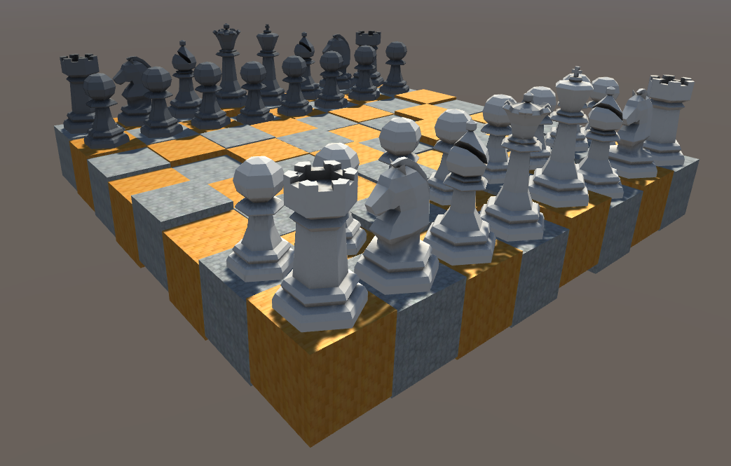
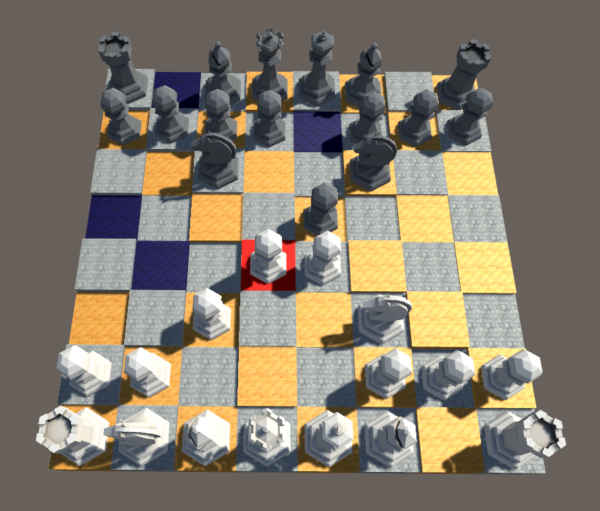
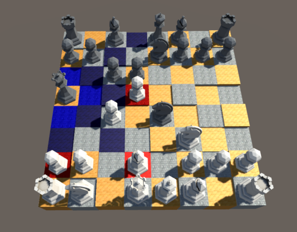
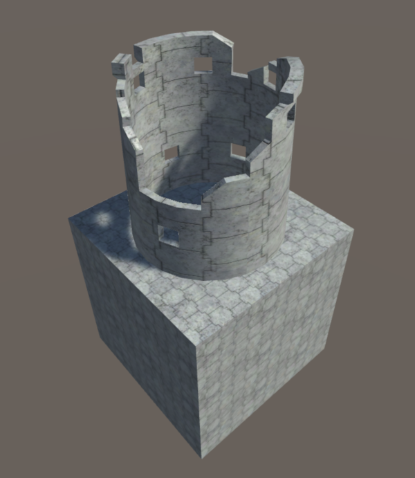
The original idea of this project was named Balanced Dungeon Chess Generator. Its goal was to create an algorithm that could generate new random chessboard, with all sorts of features, while making sure that the game was still balanced for both players.
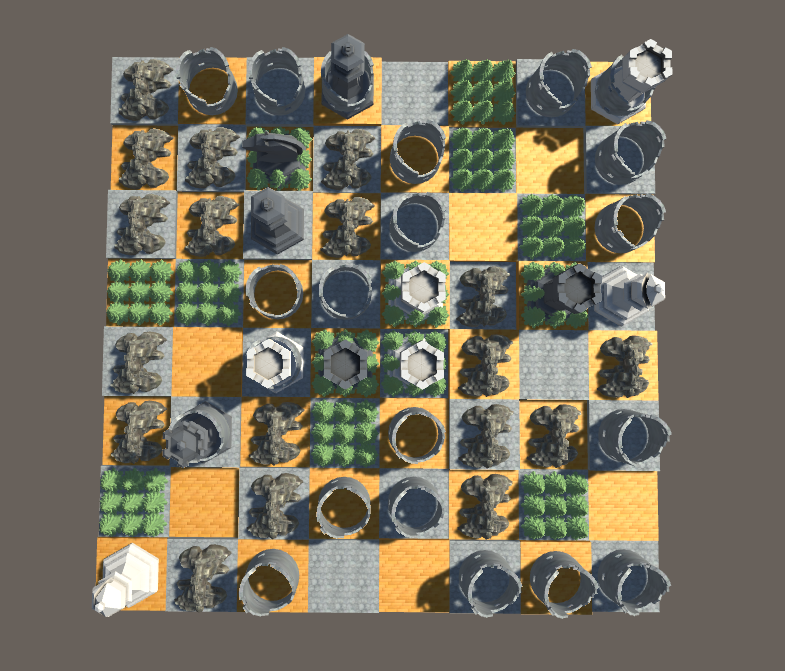
Here is a picture of what is a BDCG board state.
Creating a random chessboard isn't that hard, it only requires to put random pieces and random tiles at random places, and that's it,
we have a random board!
But the really interesting feature is to manage to create a balanced chessboard so that both players have
the same chances to win. And I think this is the feature that makes the difference between a boring board and an interesting one.
So this was the main challenge: balancing.
Plan of BDCG
So, how do we do that? How could we achieve to create a board that is balanced for both players? I mean, even a chess master would have
difficulties to be able to say if a board that he has never seen before is balanced or favored for one player, especially if we are adding new
features that he is unfamiliar with (we will talk about that later)! He would have to play from this board state again and again to start
having a feeling of who "should" (assuming both players are playing perfectly) win in this game state.
But in fact, this is exactly the idea I wanted to implement! Having a chess master that could tell whether or not the game is balanced!
So here is the plan to implement an algorithm that generates balanced boards:
1) Generate a random board state.
2) Train an agent to become a chess master on this board, for white and black.
3) Once the agent is fully trained, make the agent play a large number of games against itself.
3)a) If the win ratio is not balanced, go back to step 1).
3)b) If the win ratio is balanced, congratulation! You just created a new balanced board chess game!
We will now discuss each of these 3 points to see how to implement them and where are the challenges.
What is the best way to generate a random board state?
The main obstacle is that we may never succeed in randomly create a balanced chessboard, even if we can generate a lot of different boards!
And this is mainly due to the fact that it is possible (I am not sure, but I think it is, and we have to take into account all possibilities)
that our space of existing boards is dense with non-balanced boards so that finding a balanced board is very unlikely to happen.
In the same way as a randomly generated image is unlikely to give us the face of a recognizable person, having a random board to be a balanced board
is unlikely to happen. However, in image generation, people succeeded in finding a technique that solves this problem, so the same technique will be adapted to address our problem of board generation!
This technique is called Generative Adversarial Networks (or GAN) and the idea behind GAN, which I think is amazing, is the following:
2 neural networks are competing with each other to outclass the other network, the first network is a generator which will create "things",
and the second network is a classifier which will try to decide whether or not the "thing" created by the first network is valid or not. Both of
them are rewarded if they manage to beat the other: the first network will be rewarded if it could create a thing that the second one fails to classify
and the second will be rewarded if it successfully classifies the thing the first network created.
In image face generation, they used to train GAN with a network generating face images and a second network that was a classifier of face
images. And that gave excellent results!
For random board generation, the same process will be used.
A first network generates random boards and a second network that will be a master chess player will try to "crack" the board and win every single game on it!
If the second network wins most of the time ("most" being defined with a threshold on the winrate) then the first network will be
punished and have a bad reward. However, if the second network never manages to find an optimal strategy on this board (that's what I meant by
"cracking") then the first network will be rewarded in order to improve the number of boards of this kind!
We need a chess master algorithm: let's use AlphaGo Zero!
If you are still with me, the second network of our GAN shall be able to play state-of-the art games of chess so that
he could really determine whether or not a board of chess is balanced.
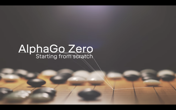
For the game of Go, DeepMind at Google already addresses this problem with the state-of-the-art algorithm AlphaGo Zero that showed stunning results in 2017 by
beating the precedent version of this algorithm, AlphaGo (that previously won against the World Champion Lee Se-dol), 100 games to 0!
There are 2 things that are absolutely amazing about this algorithm:
First, it uses Reinforcement Learning, which means that it learns from only the rules of the game and without human knowledge to supervise it.
The idea is to let the algorithm (the agent) play against itself so that it will learn from its own mistakes. This is amazing because it
allows the agent to not being lead by human knowledge and to discover its own playstyle (and therefore its own intelligence) without being
bounded by potential human mistakes and conventions.
Second, this algorithm doesn't need anything except the rules of the game. This means that it is generalist enough to be easily adapted to
other perfect-information games such as Chess!
And these are the two reasons I chose to reproduce this algorithm as the second network of the GAN.
If an agent can't take over its opponent, it is proof of a balanced game?
This is the more debatable part of the plan.
First of all, in perfect-information game theory with two players, if draws are not considered, each state of a game is either a winning state or
a losing state. This means that if both players play perfectly, one of them will always win from one fixed state of the game. This is
called Zermelo's theorem. So, as a direct consequence of this theorem, a balanced board state at Chess can't exist! Even our well known classic Chess is not balanced!
However, Chess is a really deep and complicated game. According to Shanon, there are about 10118 different possible ends for
the Chess game, which means that it is impossible to brute-force Chess to find the optimal strategy.
Given that Chess is very complicated and that Chess could end with a draw, the optimal strategy has never been found for white or black, even if
it exists! This means that a balanced board of chess on which players can compare their skills is still possible!
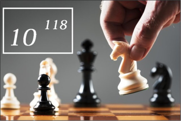
10118 is a lot! They are 1080 atoms in the visible universe.
So even if each atom could test 1 ending each second,
it would still require 1038 seconds = 1030 years to compute all possible cases!
Second, it is important to realize that it is not because one algorithm can't find the optimal strategy that the game can't be cracked. An
example of this is with AlphaZero for Go, it would be absolutely foolish for a human to try to beat it, it is almost impossible now. For this
reason, from the human referential, one might say that AlphaZero cracked Go. In the same way, and this is the most important part, it is not
because an algorithm can't crack a chessboard that it can't be cracked by another algorithm or even a human! This means that if the
second network of the GAN can't find an overwhelming strategy, it doesn't mean that the game is balanced.
Third, this might seems like bad news, but if we manage to create an algorithm as strong at Chess as AlphaZero is, and if that algorithm can't manage to crack a board state, then that means, with high probability, that a human couldn't crack it either! So we can still say
that "using AlphaZero as a heuristic of how balanced a board state is" is still a good idea!
Finally, there is one more problem to solve: how to decide if AlphaZero has converged and cracked a board state? After some time, if the win rate of one player is around or above 90%, we could assume that the algorithm cracked the board state. But what if after some time, the win
rate of both players is still around 50%? Does this mean that the board state is balanced? Or does this mean that the algorithm didn't have
enough time to converge? This is a really important and annoying question. In theory, it is not possible to know. But in practice, we could average the times that the algorithm needed to converge when it converged to estimate a duration after which it is very unlikely to converge anymore.
Why it didn't work like planned ...!
Unfortunately, I never succeed to make work this beautiful algorithm. I still think it would work, but I just used the wrong tools and this
totally prevented me from succeeding.
I think my biggest mistake was to want to have a 3D representation of a board state in order to be able to easily understand what was going on and debug. However, to do that I decided to use Unity as it's really convenient for 3D games. But what I didn't think of was that the combination of Unity + C# made the importation of a DeepLearning framework into the project really complicated. I tried to import one, but I didn't succeed. However, I didn't stop here. I decided that I would create my own DeepLearning framework. This time I
succeeded, and it was an amazing learning experience. However, I didn't realize that C# was such a slow language,
because of its intensive uses of references. Contrary to C++ it is not an Oriented Object Language but a Reference Oriented Language.
I know that if a lot of Machine Learning framework are fast it is because they are intensively using GPU for computing matrix products. I could have tried to do the same thing in C#, but as this project is mainly a training project I didn't want to spend too much time and effort to reinvent the wheel if this doesn't teach me anything.
In the end, the speed of my algorithm, due to the slowness of the language, is what prevented me to make my algorithm work.
If I had to do it again, I would directly start in Python :)
Code of the Chess game
Even before we start thinking about AI, we need what we call an environment. We need a place where our agents could act and evolves, and here
it will be the famous Chess game. I could have either import one, or create my own. I decided to create my own Chess game for 2 reasons.
First, I will be in control of every single detail in my implementation and this will allow me to have better adaptability to problems
and a better understanding of any situations.
Second, it will allow me to modify everything as I wish. If I want to replace all Bishops and Knights by Rooks, I can do it. If I want all
Pawns to move like Queens, I can do it. If I want my opponent to skip its 3 first turns, I can still do it. And this is as fun as useful! <3
For all of these reasons, coding my own Chess game was a necessity.
Main Goals of the Chess game
While developing the code of this Chess games, I had several objectives in mind.
First of all, I really wanted my code to be Data-Driven. I wanted to be able to easily change all parameters of a game
without having to go fetch the right place inside the code and hard-change it, I just wanted to press a button to do it. To do that,
Blueprints of Unity are really convenient so I intensively used them. This allowed me to code the code of the game once while having
lots of different "games" I could play with.
Second, I wanted the interface for the human player to be as intuitive and accessible as possible. I didn't want the numeric
interface to be a barrier to play this game.
Third, I wanted to be able to rapidly swap a human player with a bot or an AI. (a bot is a hard-coded agent while an AI is a machine
Learning agent)
Here we can instantly see where the knight and the queen can go and where they can capture.
Global architecture
As always when I am developing games, I am trying to create a class for everything that I can name in the game. I am then connecting them
together in the way that seems the more logical. So this is how I introduced the Board, Tile, Piece, Move, Player and Camera classes.
However I was needed some others classes to link them together, this is why I have the GameManager that takes care about all instances
used in the game, the PieceManager that takes cares about the Pieces that are instantiated in the game and the VictoryManager that
decide whether or not the game is ended.
The Piece and Move classes
All Pieces have moves, and it's them which define what the Piece can do. As an instance, it exists a vertical and horizontal move that
can go as far as possible in these directions, as it exists a diagonal move that can go only one tile away.
All Chess pieces (Pawns, Bishops, Knights, Rooks, Queens, and Kings) are Pieces (really? :o), but I have chosen not to give them specific
classes. For instance, I didn't make a Rook or Pawn class that would inherit from the Piece class. Instead of this, I have chosen to use
a Composition approach instead of an Inheritance approach. It is more flexible as a Piece is now entirely describes by the Moves it owns.
So a rook is a rook because it can moves horizontally and vertically of any number of cases it wants, it is not a rook because it is labeled like
it. As I said early, it offers more possibilities because if we want to interact with our Piece moves, we can easily do so without having
to create another class! This way we can easily imagine a Rook-Knight, or even promote a Piece in the middle of the game into a Rook-Knight!
I think it would be fun :)
However, Piece still has a labeled attribute that tells whether the Piece is intended to be a PAWN/BISHOP/KNIGHT/ROOK/QUEEN/KING for convenience
purposes.
The Player class
The GameManager owns 2 Player instances, one for white and one for black. I wanted the GameManager to interact in the same way with Players regardless of the Player being a human or an AI. For this reason, there are several classes that inherit from the Player class such as HumanPlayer, RandomPlayer, and NeuralNetworkPlayer. And all of them implement the Play method that takes in parameters the board state and gives back a Play as a result.
The Tile class
Maybe you wonder why do we need a Tile class? After all, all the Tiles in Chess are the same, we can go on either one without differences
(except for Bishops!). So why a Tile class?
If you remember well, the ultimate goal was to generate a new board state, and to achieve that, one of my ideas was to allow the Chess game
to have different types of tiles! I started with 4 types:
- The Mountain: you can't stand or cross this tile, never!
- The Forest: you can go and stand on this tile, but you can cross it if you weren't already on it!
- The Dungeon: you can move normally on this tile. However, if you capture an opponent piece that was already on a Dungeon Tile, the opponent
piece would capture your piece back!
- The Nothing Tile: this is the default Tile that does nothing special :)
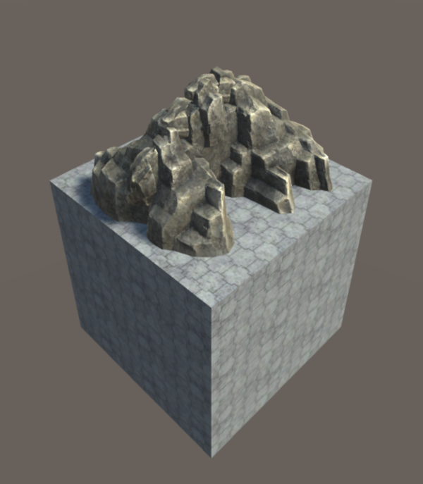
Mountain
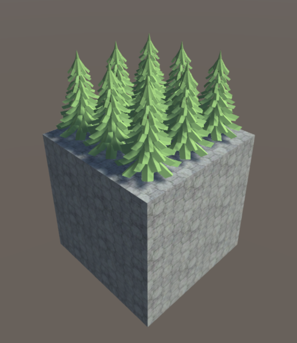
Forest
Dungeon
Here are the different Tiles types.
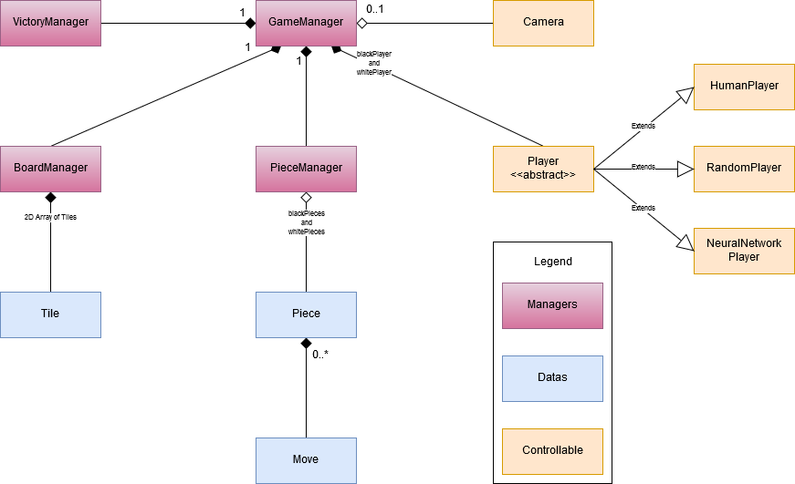
Here is an UML to visualize the whole architecture.
The Replay feature
Even before I started programming any AI, I knew I would need to be able to observe what the AI was doing, in order to debug and understand it. I didn't want to have to read text representations of a game of chess, because they are just unreadable to me!
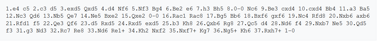
As you can see, it's not really ... convenient.
For this reason, I started implementing the Replay feature.
Game representation
In principle a Replay isn't that hard, you just need to describe an initial situation and gives all the plays (as pair of board positions) of
the game, one by one, and you would have a perfectly fine Replay feature! (Just avoid to give all states after each plays because it would be
extremely resource intensive!)
The difficulty lies, not in the model of the game that could be really easily described, but in the view of the game. In my Chess code, the
view of the game is how I represent the board and the pieces of the game to the screen: it is the ensemble of the 3D assets that are used to
display the game to the screen, like the shape of pawns, bishops and so on.
Because I wanted not being restrained to a certain set of types of pieces, I also needed to refer to the view a piece was attached to. And this
was a bit more difficult as it wasn't just an enumeration, it was the id of an entire asset. Fortunately, the serialization feature of C# manages
this easily! But it leads to other difficulties! ...
Serialization
The serialization of C# is really easy to use, you just give it an object, and it will entirely serialize it for you into a json string.
Except that it doesn't handle abstract classes and inheritance and List of List and reference cycles. And guess what? A GameObject (the
thing you really care to serialize) is just a container that posses a lot of Components, and a Component is ... an abstract class! So this
means that in the end, you can't serialize anything easily ...
To tackle this problem, we have to use a technique named Data Extraction. The idea is that for a given class, you will create a structure
whose only purpose is to contain the data of your class. And then your class, which you can't serialize, will reference the structure you
have created. And you can serialize this structure. You then only need to have a conversion function that can generate your class from
your structure and reciprocally.
I think this is a bad design as it forces you to duplicate a lot of code and have 2 classes that represent the same thing, which is never
a good idea. However, I needed that technique and I think it was the best solution overall. It could even have advantages if we want
to optimize cache memory by putting all the structure in the same memory space so that we can iterate over them very quickly! (But this
is not something we can do in C#, it's more of C++ stuff.)
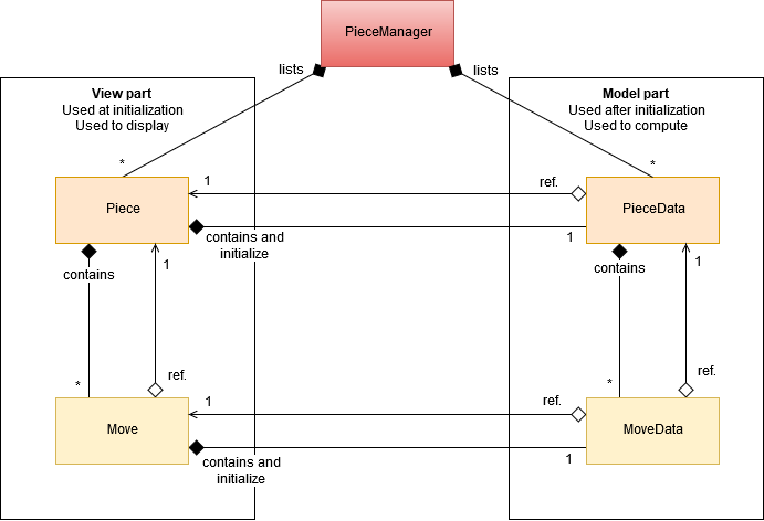
Here is a UML diagram that summaries the Data Extraction technique.
And here we can see what it finally looks like!
It is a Replay of a game of myself against myself :)
Camera
To have a good replay feature, I was thinking that a good camera that allows us to have good vision angles on the board was also a necessity.
So this is what the camera look like:
The Camera movements.
The Neural Network API
As I didn't succeed to import a Machine Learning API such as Keras, TensorFlow, SciSharp, TensorSharp or Numpy, I decided to code my own
API in Machine Learning! Overall, I am glad it happened because it allowed me to learn a lot of things I wouldn't have discovered
otherwise :)
Numpy Code
The Numpy code could be easily summarized in 1 class, the NDarray class. Because Numpy is all about being able to represent arrays of data
of any dimension. In fact, the strength of Numpy is that it does have 1 class that can at the same time represent, with numerical efficiency,
a single number, a flat array or even an n-dimensional array! And this is where all the challenge is!
First of all, the NDarray class has to be a generic class NDarray
Second, to be able to represent any kind of data with only 1 class, a good technique was to use both a single fixed size array paired with another class that would tell what the shape of the fixed size array is. And this second class is named Shape. A Shape is just a list of integers
which all describe the size of their dimension. As an instance, a {2, 3, 4} list for a Shape would represent a 3 dimensional array with 2
numbers in the first dimension, 3 in the second and 4 in the last dimension.
Third, as Numpy is the basic brick of our implementation, it is important that it is as easy to use as possible. That's why I spent time at
developing user friendly getters and setters and functions such as :
- a flat getter: my3DNDarray[42] will return the 43rd element of this 3D array starting from the element [0, 0, 0] and starting incrementing by
the last dimension.
- a full dimension getter: my3DNDarray[1, 2, 3] will return the element which is 2nd in the first dimension, 3rd in the second dimension
and 4th in the last dimension.
- a flat setter.
- a full dimension setter.
*** An important point here is that these getters and setters had to be well coded so that adjacent elements in the N dimensional array
would also be adjacent in the flat array representation so that we prevent memory jumps as much as possible. ***
- a bidirectional conversion with Lists.
- a bidirectional conversion with arrays.
- a lot of different constructors.
- copy constructor.
- a flatten function (just have to change the Shape, very easy :D).
- ToString, very useful for debugging.
- the Transpose function.
- the Fill function.
- a Map function that applies a delegate function to all elements of the array.
Then, using C++ templates I would have been able to continue, however as C# genericity is not as strong, I had to create a subclass NDarrayF for
float only that would be able to implement the others functions I needed. Happily, most of my NDarray were NDarrayF anyway! :)
- Max and Min.
- Argmax and Argmin.
- Plus, Minus, Mult, Divide, element to element.
- Outer product.
- Dot product, for 1D-arrays and 2D-arrays.
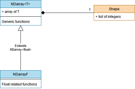
Here is a UML diagram that summaries the Numpy API.
Keras Code
Keras is a TensorFlow API that allows to easily models Deep Learning architecture.
Now that the Numpy part is completed, it is possible to start coding Keras! :)
I decided to focus on the ModelSequential part of the Keras API for this project as it was the most suitable.
Brief explanation of the ModelSequential of Keras
The goal of a Deep Learning algorithm (a network), and so of a ModelSequential, is to approximate a function. No matter how complicated
(almost) the function is, a good Deep Learning network is supposed to be able at some point to represent it! It is especially interesting
to use a Deep neural network when the function to approximate isn't linear, because else it is easy and we should use other methods!
In our case, the function we try to approximate is the one that gives the best play to play for a given board state of chess.
The plan in a ModelSequential is to have a succession of layers so that each output of a layer will be the input of the next layer.
This means that you are giving an input to your model, it will give it to the first layer which will compute its own output, give this output
to the next layer and so on until the last layer that will compute the final result of the model.
Then, in the training phase, the final output is compared to an expected output and the difference (according to some metrics) is called the loss.
This loss is then used in the backpropagation part. The role of the backpropagation part is to update the parameters of all layers so that
the next time the model is given the same input it will compute a final result that is closer to the expected output than before. To do that
the technique of the Gradient Descent is used. The Gradient Descent will compute how to modify the parameters thanks to a local derivative,
that the layer can compute itself, and the derivative of the next layer using the Chain Rule. As each layer needs for the next layer, we are
computing this from end to start, this is why it is called the backpropagation of the gradient.
Everything is a layer!
So as I said, we have layers! But what are the purposes of these layers? So, we have a few of them :
- the Input Layer. This one is just used for code conveniences, it doesn't do anything. It is used as the first layer of the model.
- the Flatten Layer. Its role is to flatten its input to allow the next layers to work easily on it.
- the Dense Layer. This is where the real work happens. A Dense Layer is simulating a number N of neurons. Each neuron is a linear combination
of the input using the weights of each neuron and adding a bias. This means that a Dense Layer is composed of a matrix of weights of size (N, D)
where N is the number of neurons and D the size of the input, and of a vector of bias of size N. The output of a Dense Layer will be a vector A of
size N where A[i] = sumj(Weight[i, j] * Input[j]) + Bias[i].
It is interesting to note that if a model was only constituted of Dense Layer like describe until now, it wouldn't be really helpful as a
composition of linear combination is still a linear combination! So we could have as many Dense Layer as we like, it would still be equivalent to
a single Dense Layer with weights and bias being the result of the combination of all layers, what a waste of time!
For this reason, after computing the linear combination, non-linearity functions (also named activation function) are being introduced that
will allow the network to also learn non-linear function. After computing A, we will then compute Z defined by
Z[i] = ActivationFunction(A[i]).
- the Softmax Layer. At the end of the network, we are expecting an array of probabilities, which are all representing the probability of each
play to be the best to chose. However, the output of a Dense Layer is not normalized. We are then using the Softmax Layer that can normalize
an array so that it sum-up to 1. To do that we are pre-computing S = sumi(eInput[i]). And then we can compute the output
which is Output[i] = eInput[i] / S.
However, there is a little problem here. If the Inputs are very larges, eInput will be even more large, easily exceeded the maximum
number for whatever float/int/double we are using. To do that, there is a cute little trick :) We can first observe that
eInput[i] / S = (eInput[i] * D) / (S * D) = eInput[i] + ln(D) / sumi(eInput[i] + ln(D))
for all D. As it's true for all D, we can remove the logarithme, as we only have to chose D' = ln(D) and it would still be true. The
interest of this is that if D' is negative and big enough, the exponential won't explode and it won't make a number overflow! In practice
we chose D' = - Maxi(Input[i]).
- the Batch Normalization Layer. Its role is to normalize and center the data of an entire batch by subtracting the mean of the batch
and dividing by the variance of the batch. It does have a lot of advantages, and that's why we are using it after almost every other layers:
Improves gradient flow, allow higher learning rates, reduce dependency on initialization, and regularize. Something to add that is very
interesting is that a Batch Normalization Layer has 2 parameters, alpha and gamma, that allow the network to shift and scale back the data. As
an instance, the network could even learn how to undo the normalization and the centering if it wanted too, and this what gives the flexibility
to this layer.
- the Convolutional Layer. It is the core layer for computing stuff on images and othes data where local neirghborhood is very important, such
as chessboards! A Convolutional Layer is constituted of filters. Each filter will constitute a 2 dimensional array using its own kernel by doing
a convolutional product between the kernel and the input image. The results are then concatenated in a 3 dimensional array, which is the
final output of the layer. In a way, it is very similar to a Dense Layer, except that neurons are only connected to a local part of the inputs
and that all neurons share the same parameters. This means that every location of the input is treated identically. It is the Convolutional Layers
that made image recognition to be as successful as it is today.
The forward pass
The forward pass is what I describe just above. It is the first pass where layers are computing what they are meant to compute.
In the testing phase of the neural network, we are only doing the forward pass to get the prediction of the neural network.
In the training phase of the neural network, we are also doing the forward pass to be able to compute the loss from the prediction of
the neural network and the expected output. And we will use that loss for the backward pass.
The backward pass
The backward pass is, as I explained earlier, the pass where we are updating the parameters of the layers to get better results next time.
It is important to note that only layers themselves can know how to compute the backward pass, which means that when we are coding a layer we
always need to implement both the forward and the backward pass.
As an instance, the parameters in the Dense Layer are the weights matrice and the bias vector which we will update using the Chain Rule and
the gradient of the next layer. We will also need to compute the gradient of the influence of the input over the loss so that we can propagate
this value for the precedent layer.
Which activation function?
As I explained above, Dense Layers need an activation function.
At first, I didn't know how to chose between all these activation functions: Sigmoid, Hyperbolic Tangent, ReLu, LeakyRelu, ELU and so on.
The Sigmoid and the Vanishing Gradient problem
I have chosen the Sigmoid function as it was the first to appear in the literature.
Sigmoid(x) = 1 / (1 + e-x)
However, when I tried my network for the first time, I quickly noticed that my weights weren't updated. I tried for a while to understand
the reason for this annoying phenomenon and after looking online I realize that it was because of the Vanishing Gradient problem.
When we look at the Sigmoid function and it's derivative it looks like this:
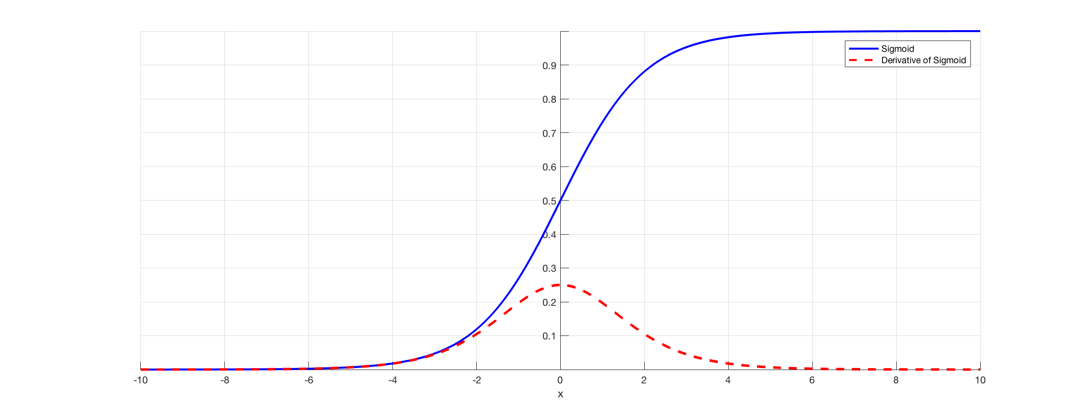
In blue the Sigmoid and in red it's derivative. We can see that the derivative is extremely small on the edges.
And the problem cause is that on the edges, that is to say before -4 or after 4, the derivative is extremely small. And as we might have many
Dense Layer in our network, the gradient will decrease exponentially fast, until it reaches zero with numerical approximations. And at that point,
the network stops learning.
This is why it is mainly recommended today to use a Rectified Linear Unit (ReLu) as the activation function.
The ReLu and the Dying Neuron problem
The Rectified Linear Unit (ReLu) has a lot of advantages over the Sigmoid function.
ReLu(x) = (x > 0) ? x : 0 = max(0, x)
First of all, it is much more easy to compute as we only need one max operator where for the Sigmoid we had to compute an exponential which is
very expensive.
Second, on the positive part, the gradient is always equal to 1, this means that we won't decrease the gradient at all, no matter how many
layers we use as multiplying by 1 is the identity! So the Vanishing Gradient problem is solved.
Third, ReLu is known for converging much faster than Sigmoid and TanH in practice.
However, on the negative part, the derivative of ReLu is always 0. This means that if we always get a negative input, we will always output 0
and will always shut down the gradient. Which is a good thing as this non-continuity is the source of non-linearity for ReLu, but it will
totally prevent the network from learning in these areas of the network. This is called the Dying Neuron problem.
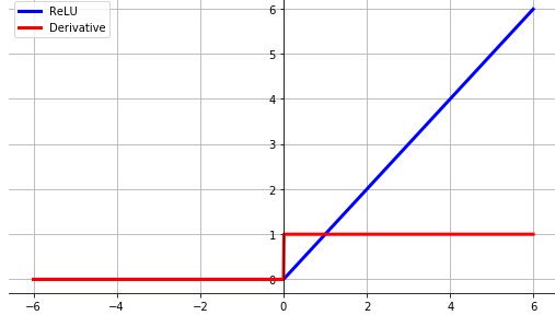
In blue the ReLu function and in red it's derivative.
The final activation function: LeakyRelu
Having a large part of our network not being trained is not really what we want. So in order to prevent this issue, they are several
solutions :
- We could use a better initialization where we would add a voluntary positive bias on the bias so that most of our input of ReLu are positive
- We could use somewhat of an upgrade of ReLu: LeakyRelu. LeakyRelu is exactly as ReLu except in the negative part where it let pass a small
part of the gradient.
LeakyRelu(x) = (x > 0) ? x : ax = max(ax, x) where a is often chosed as a = 0.01.
LeakyRelu has all the advantages of ReLu except that it also let pass through the gradient in the negative part. It is the solution I
have chosen, and it worked perfectly fine!
However, it is even possible to go further with a parametrized LeakyRelu where the parameter a is learned in the backpropagation pass, or even
ELU but I won't describe it here.
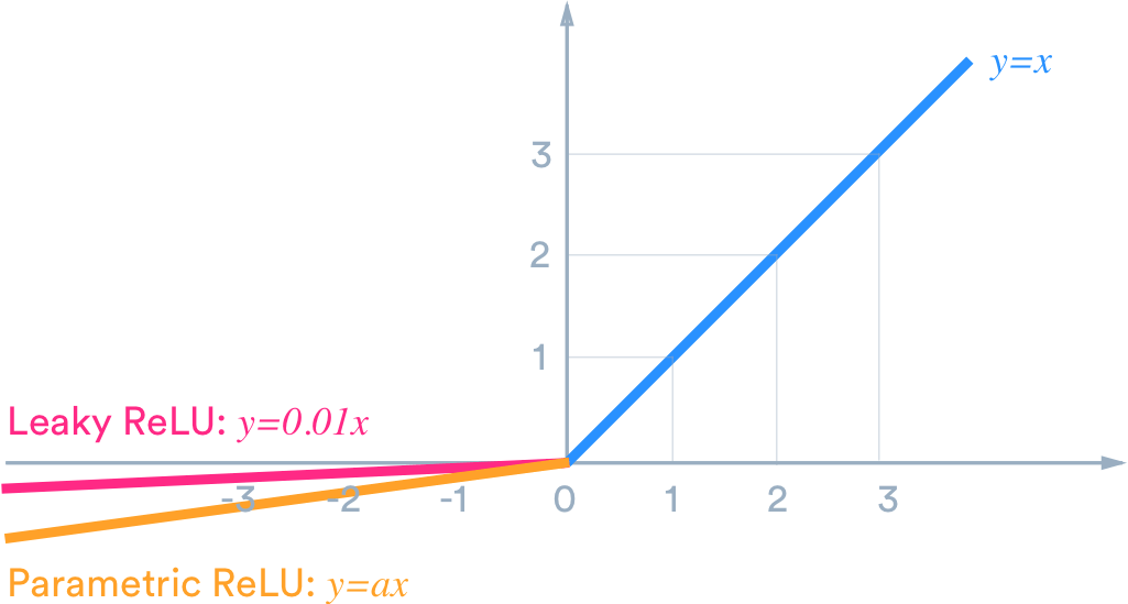
LeakyRelu and ParametricReLu.
First Neural Network
I was so happy, I had designed a Neural Network architecture and it was working fine, as I already tested it on easier problems. I was really
excited to finally be able to test it for real on this Chess game! I knew something was missing because AlphaGo Zero was much more complicated
but I wanted to see what a simple neural net could learn from it and what was its limits.
To do that, I needed 2 things :
- first a way of representing a chessboard that my network could understand.
- second a way of representing the play my network had chosen so that my chess algorithm could understand it.
The GameState
I already had all the useful information to give to the neural network, I only needed to order them in the good way. The GameState class was
designed for this purpose.
Problem : A variable number of parameters
So, what are the pertinent information to give? We will need to know where are the pieces, where are the obstacles such as forest, mountains and
dungeons (I still wanted that my network could learn this homemade features, because why not :)), who is the current player, and what is the
current turn (as I had to set up a maximum turn number to prevent draws from going infinite). Ok, cool.
But a neural network is really good at understanding a fixed number of features. However here, we don't really know in advance how many pieces
and how many obstacles we will have because maybe they will be captured during the game! I wanted to give the network 2 parameters by pieces,
the column indices and the line indices because it seemed like the easiest way of describing a position to me, but by doing that I would have
nbParams = 2 * (nbPieces + nbObstacles) which is a variable number. I could have used a maximum number of parameters and then not using the
parameters that weren't useful, it could have worked. But what if I needed to create a new piece during the game because of some special event
or something else? I wasn't convinced by this solution.
The solution: The planes
After looking inside the AlphaGo Zero papers I learned the solution. It is possible to use what is called a plane. A plane is a set of
booleans parameters as big as the board which is associated with a feature. When the feature is present on a tile, the boolean is set to true, else
it is set to false. And this is an amazing solution!
Even if it is expensive, as it often as a lot of zeros for only some ones, it can ensure that if we have a plane for each possible existing
piece and obstacle we could represent as many pieces and obstacles as we want! Problem solved!
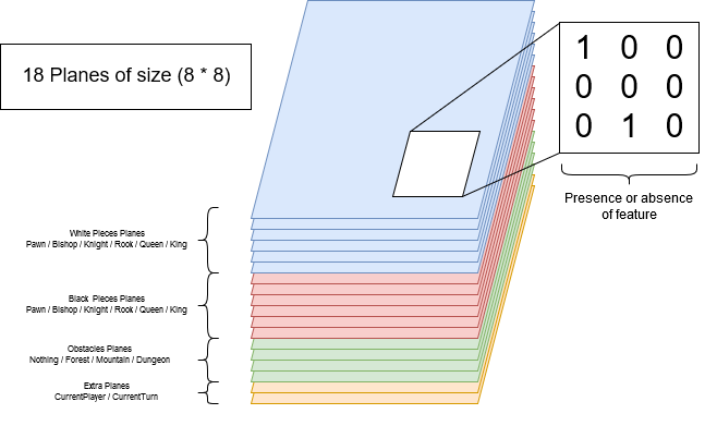
Here is a diagram of the plane representation of a GameState.
Representation of a Play
It is much easier to represent a play than a piece, as we know in advance that we will only have one play, always. This means that our
neural network is just a classifier that takes a GameState in input and will classify the best play to make between all possibles plays.
We only have a good way of representing all the possible plays.
A good way to do this is by specifying the tile from which the piece must start and then specifying the kind of movement this piece is using.
A queen has 4 directions with 7 locations on each on an 8x8 board for a total of 24 possible movements. At this, we must add the 8
possibles movements of the knight for a total of (4 * 7) + 8 = 36 possible movements. This means that if we have 8 * 8 = 64 starting
positions, we have a total of 36 * 64 = 2304 possible plays! And so our neural network will have to have 2304 outputs.
The above version is what DeepMind implemented for their version of AlphaZero for Chess. However, I wanted to be a little more flexible as I might
want to add new exotic moves. For this reason, I decided to represent a play with it's starting position and it's ending position for
(8 * 8) * (8 * 8) = 4096 outputs. This version is slower to train as they are more class to chose between, but it is the cost to pay for
versatility.
No matter the version we chose, we still need a conversion function between the indices of the play that will give the neural network and the
play (with 2 parameters) we are looking for. For this, we just have to order all the plays.
What if the Play chosen by the Neural Network is not a valid Play?
If this happens, this play is just ignored and we are then considering the second best play. We are doing this until one is valid! Hopefully, there is always a play to do if we are not checkmated!
The final output of the Neural Network
In the AlphaGo Zero paper, they are training simultaneously the neural network to tell the percentage of chance of the current player to win in this current situation. I found that very interesting so I keep it. To do that, we only need to add the last output to our 4096 and it's role will just to print the expected winrate.
Always start simple
As I knew that would probably not succeed on the first try, and as I didn't want to lose time in computation if it wasn't going to work, I
decided to design smallest chessboard so that I can test and try easier and faster on them.
Here what they look like:
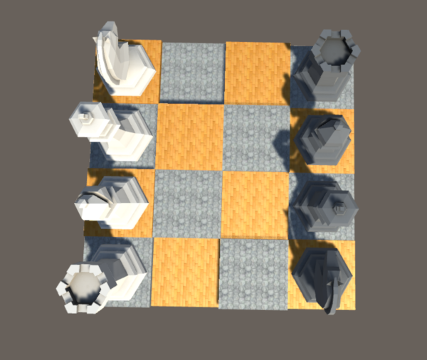
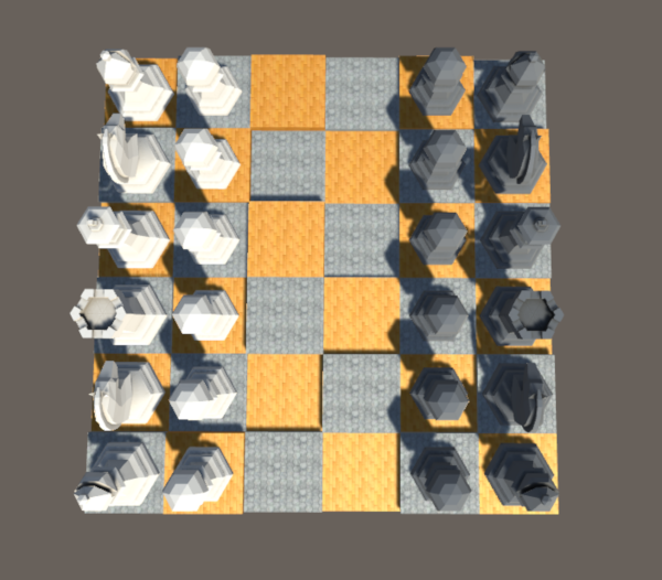
The 4x4 and the 6x6 chessboards!
Did someone talk about an expected output?
Ok, so everything was ready. Network? Ready! Input? Ready! Output? Ready!
But then I just went to the computation of the loss function. You know, in order that the network can train ... And I realized that I didn't know
how to train the network. I mean I know how to use backpropagation, but to converge towards what? What was the expected output that the
network should converge towards?
Well, from the previous architecture, we just can't calculate or even approximate it. And that's why Go and Chess are such challenging
problems!
Then I understand the utility of the Monte-Carlo-Tree-Search.
A heuristic of the expected output: Monte-Carlo-Tree-Search (MCTS)
In order to help us compute the expected output (which is what is are all praying for!), we will use an MCTS!
An MCTS is a graph search algorithm. Its goal is to find the best node of the game graph by using a theoretical optimal compromise between
exploration and exploitation. Ok. It is a lot of information, let's break it down.
A game graph of chess is a graph where each node represents a board of chess with its pieces. From a node, which is a board state, we have a
finite number of possible moves. Each of these moves will result in a different board state, which is represented by a different node. Each of
these different nodes is called a successor of the first node and is linked to it.
This graph search algorithm has the objective to search inside the game graph describe above the best child node of the current
game state. How to choose the "Best", which stands for "it is the best move to do", will be described later :)
Exploration and Exploitation
The MCTS could be seen as a generalization (or extension) of the k-bandit machines problem, which is a very well known problem.
In the k-bandit machines problem, we are facing k bandit machines which are slot machines. We have a finite number of turns n. At each turn
we can activate only one machine. Each machine i has it's unknown probability pi of rewarding us. What is the best way of
activating the machines in order to maximize the number of rewards? I love this problem! :)
We can immediately notice something:
- first, it might seem intuitive to try to activate as often as possible the machine that seems to have better efficiency (=
numberOfRewards / numberOfActivations). This is the exploitation part.
- second, how is it possible to know which machine has the best efficiency without trying them all? This is the exploration part.
- third, how decide that the machine we have chosen is really the most efficient? We might have been the victim of a bad sample and have
chosen a sub-optimal machine.
To summarize, we have at each turn to chose between 2 strategies: Exploration and Exploitation. And the balance between these two is the
heart of the problem.
How works an MCTS?
Now that we are understanding what are the stakes behind Exploration and Exploitation, let's dive down into the architecture of an MCTS.
At the start of the MCTS, the graph is initialized with only the current state of the game as the root of our graph.
A leaf of this graph (which is a tree) is either a final configuration (someone win or it's a draw) or a state from which we haven't launched
any simulations.
In each node of this graph, we will store the number of times we have simulated this node, named N, and the number of times we have won from these
simulations, named W.
An MCTS is a loop that can be broken down into several parts:
- Selection.
- Expansion.
- Simulation.
- Backpropagation. (again!)
We will get out of this loop when we consider that we have gathered enough information to make a good decision.
In the AlphaZero algorithm, they have chosen to make 800 simulations before getting out.
At the end of the MCTS loop, we will have an N and an M for each of the children of the current state of the game. These N and M are forming a
heuristic of how likely we are going to win by choosing this move. And this is exactly what we were looking for our Neural Network. This is
going to be our expected output!
Selection
This is the most important part.
It used a heuristic for choosing between several nodes. The choice of this heuristic is crucial and could make a huge difference between a good
and a not as good MCTS. So, we need to choose a heuristic. But for now, let's assume we have one.
In this part, we will choose which node will be the next to be expanded. For this we start from the root of our tree, applying our heuristic
to chose the best child of this node to select, then if we aren't to a leaf of the graph we continue applying our heuristic until we get to a
leaf. This leaf is then given to the Expansion part.
Expansion
In this part, we will expand the node we have chosen in the Selection part. For this, we will create a node for each of the children of this node's configuration. We then chose a node between all these children using the same heuristic as before.
Simulation
From the chosen node, we will simulate an entire game until its end. All the plays of the game are chosen randomly and uniformly. The consecutive states of this game aren't stored in the graph of the MCTS. When we reach the end of the game, we store the result.
Backpropagation.
The result will then be backpropagated among all the nodes until the root of the graph, updating all the N and W. As an instance, if the final node has N = 0 and W = 0 (so it was the first simulation) and we win, we will now have N = 1 and W = 1. The parent of this node would have its own N and W, let's say N = 3 and W = 2 and we will update them accordingly: N = 4 and W = 3. And we do that until we reach the root of the graph.
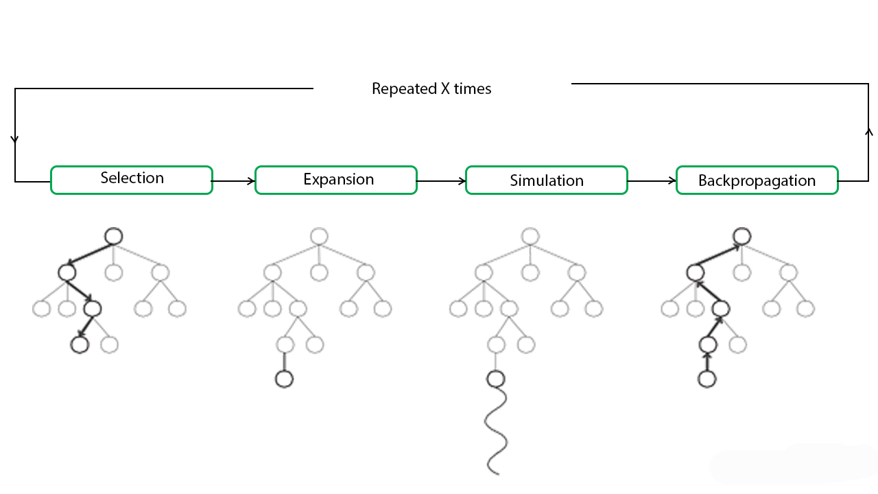
Here a diagram of how an MCTS works.
The Heuristics
Upper Confidence Bound (UCB)
We have a number N of options named A1, A2, ..., AN and we want to choose the option i that have the best
true efficiency/mean Qi. I am saying "true" because we don't know this true efficiency Q. What we know about each option is the
sample efficiency/mean Q'i = Wi / Ni.
The idea behind UCB is to compute a upper confidence bound Ui (hence the name!) such that
Qi <= Q'i + Ui with a very high probability. Once we have computed the Ui, we greedily take
the action that maximizes Q'i + Ui, and that's it!
However, you could argue: we know that Qi is not bigger than Q'i + Ui but maybe it is lower than
Q'i so we would stick to an action that has a terrible true efficiency! Yes, but no. This paradigm is called Optimism in the face
of uncertainty. The trick is that maybe the real efficiency Qi is lower than we think, but this just means we are "victim" of
a favorable variance for this action, and we should keep going on it for as long as we are lucky! Once we will get back to the harsh reality
the algorithm will naturally switch to another better upper bound confidence to keep optimizing our gains.
Ok! Great! But how do we compute Ui at each step?
You just have to apply this formula at time t: Ui(t) = sqrt(2 * log(t) / Ni)
Great ... But why? It is just the result of the application of Hoeffding's Inequality. Hoeffding's Inequality says that:
P[E[X] > Xmeant + u] <= e-2tu2 with X being a random variable and Xmeant
being the mean gain for t samples of X and u is a scalar. Applying this to our problem we get:
P[Qi > Q'i + Ui] <= e-2NiUi2 with t the number of times we
have tried this action.
T = e-2NiUi2 is a threshold that can be as small as we want. We would like this threshold to
be smaller when we have more informations over the action (when t grows), so we will set T = 1 / t4. So we have:
Ui(t) = sqrt(- log(T) / (2 * Ni)) = sqrt(2 * log(t) / Ni)
In the end, our decision process could be written as taking the action that maximizes
Xi = Q'i + Ui(t) = (Wi / Ni) + (sqrt(2 * log(t) / Ni))
We can see that our metric is divided into 2 parts. The first, the Q'i part, is increased when the sample mean of this action
is increasing and is therefore called the exploitation part. The second, the Ui(t) part, is increased when we didn't try this
action for a long time and is therefore called the exploration part. This is how this beautiful algorithm allows Exploitation and
Exploration to collaborate in a single equation! <3
Predictor + Upper Confidence Bound (PUCB)
OK! But we can do even better! The fact is that, for our problem of chess, we don't know anything about the actions we are going to chose
between. The fact is that we have a Neural Network that could tell us what actions are the most promising ones! And this is called a
Predictor and could be insert as a third term in our equation to converge even faster to the best action.
Here is the final version I used in my algorithm:
Xi = Q'i + Ui(t) + Pi
Where:
- Q'i = (Wi / Ni) as the Exploitation term as before
- Ui(t) = sqrt((3/2) * log(t) / Ni) if Ni > 0, otherwise 0. As the Exploration term as before.
(The constant change a bit but it is not that important.)
- Pi = (2 / Mi) * sqrt(log(t) / t) if t > 1, otherwise 2 / Mi. Where Mi is the prior
probability calculated by the neural network. It is the new Predictor term.
You can find more explanations about this algorithm here:
This new equation is really amazing because it has 2 advantages:
- according to the paper, it is as good ("good" being defined by the notion of "regret") as before even if the predictor used is the worst
possible. This is an important property as at the start, our neural network will definitely be a worst predictor!
- if the first actions are promising, this algorithm doesn't waste time trying all possibles actions. This could have been seen as a
disadvantage of the UCB version, as it always starts by testing one time all possibles actions, which could be too long. This time the heuristic
will more stick to the best options, thanks to the predictor.
This is the algorithm I chose to use in my program.
The beautiful Duality MCTS-NeuralNetwork
What is interesting to notice, is that in the end, an MCTS is just a big number of random simulations done in a kind of intelligent way and we
are just gathering all these random results to in the end greedily chose the node which has the best ratio Q = W / N. Not that much to talk
about.
However, and this is where I really think the things are absolutely amazing, DeepMind chose not to let the simulation being entirely random
but rather be decided by the trained Neural Network. So in one hand, the MCTS is providing the expected output to the Neural Network so that
it can backpropagate and train, and on the other hand, the Neural Network is providing the MCTS a prior probability for its heuristic in addition
to a good policy for choosing the plays in the simulation part! And this is, ladies and gentlemen, by this beautiful duality, how AlphaZero
cracked Go, Chess and Shogi!
Conclusion
I did this project in order to learn as much as possible in Machine Learning and Neural Networks and to show my motivation to a certain company
that I wished to join. I think that even all the difficulties that I met, it was an amazing experience that really teaches me the fundamentals
of Neural Networks. This project was half engineering and half research, which is why I really enjoyed it. What's more, I am happy because even
if most of it was based on work of others (AlphaZero), I didn't just copy them but expanded their work to something that was never made before
and this perspective was what motivates me the most! :)
If you want to see the source code:
Get In Touch
